After creating anatomical and functional data in normalized space, workflows can be specified and executed that perform statistical analysis of the data. The Group-GLM workflow allows to specify which normalized VTC files to use per subject in order to run group-level random or fixed effects GLM analyses. Furthermore, contrasts can be defined that will be used to calculate and overlay desired statistical maps. The specified workflows simplify substantially the setup of multi-subject GLM analyses since multi-study design matrix files are build automatically.
In order to define a statistics workflow, the Statistics Workflow icon in the main toolbar of the Data Analysis Manager window can be used (see snapshot below). Alternatively the Add button in the Workflows tab can be used after selecting the "Group-GLM" entry in the Workflows selection box on the left side of the Add button (see snapshot below).
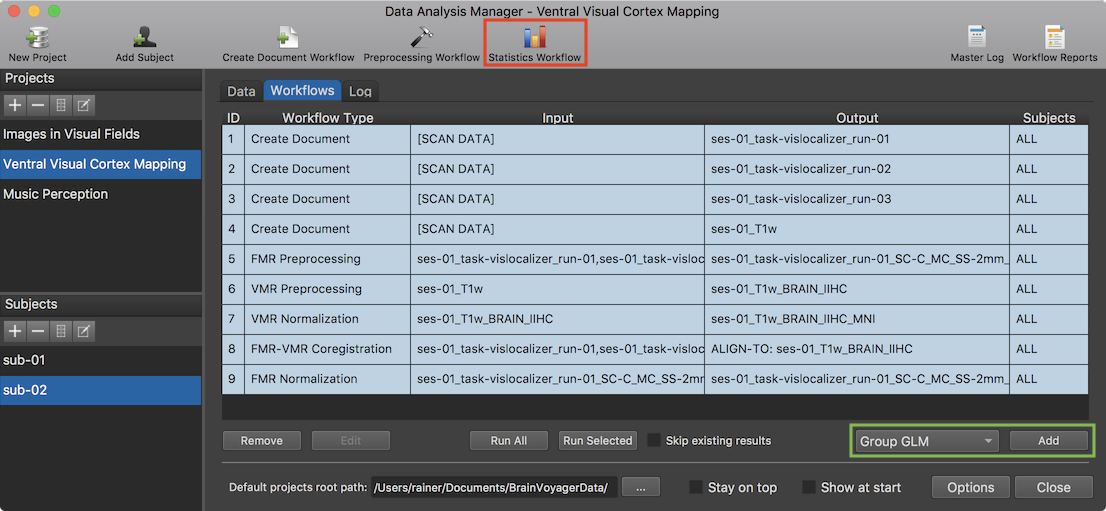
After clicking the Statistics Workflow icon (or the Add button after selecting the Group-GLM item in the Workflow list, see green rectangle), the Group-GLM Workflow dialog will appear (see screenshot below). The dialog contains two tabs, the Data and Contrasts and Options tab. The dialog will select the TAL space or MNI space option (right upper section) automatically depending on which normalization space had been used when creating the normalized functional VTC data. If data sets for both spaces are available, one can select which space should be used for the defined workflow. The Functional data sets field of the Data and Contrasts tab allows to select the VTC data sets that should be included for each subject. When entering the dialog, the first data set is selected as default. In the screenshot below all three data sets (runs) have been selected and will thus be used for group statistical analysis for each subject.
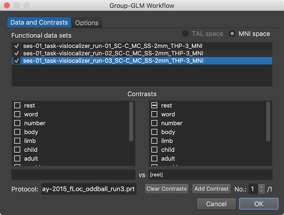
The selected VTC data sets (runs) belonging to the same subject are concatenated, i.e. subject-specific beta values are estimated as fixed effects when running group-level GLM analysis. It is also required that the protocols for the included runs need to contain the same conditions. This can be verified by selecting the included functional data sets and checking that the condition names shown in the two selection boxes in the Contrasts field are the same and displayed also in the same order for all runs. The name of the protocol associated with the selected functional data set (run) is retrieved and shown for the first subject in the Protocol field.
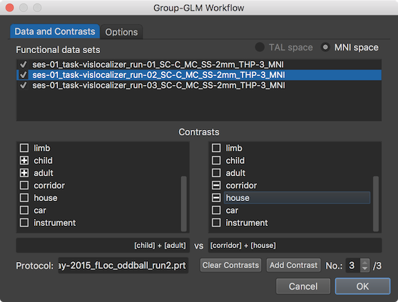
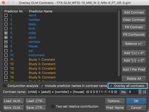
The condition names from the displayed protocol are shown in the left condition selection box and right condition selection box with a check box on the left side of each name. These two selection boxes can be used to define contrasts that will be evaluated and displayed as volume maps after calculating the group-level GLM. For the example experiment, 3 contrasts have been defined as can be seen on the right side of the contrast No. spin box, here the "/3" text. The Add Contrast button can be used to add a contrast and the Clear Contrasts button can be used to remove all but one empty contrast. A contrast is filled by checking condition names on the left side; note that the plus-selected condition names appear in the left contrast name field. In the snapshot above, the two conditions "child" and "adult" have been plus-selected (left side) and the respective condition names appear in the left contrast name field ("[child] +[adult]"). If no condition name is selected in the right condition selection box, the plus-selected conditions are compared to the baseline. This is indicated by a selected first condition in the right box (usually the baseline condition such as "rest" or "fixation") if a new empty contrast is added (independent whether the first condition is dropped from the design matrix, see below). If the selected conditions on the left side should be contrasted with specific other conditions, the desired condition names need to be selected in the right condition selection box. In the example contrast shown above, the "corridor" and "house" conditions are "minus-selected" and shown in the right contrast name field ("[corridor] + [house]"). Note that the program automatically balances the specified contrast in case that an unequal number of conditions is selected in the left and right selection box.
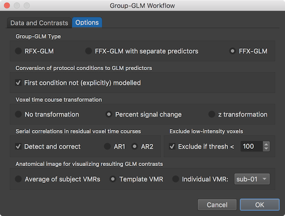
The group-GLM workflow can be customized using the settings in the Options tab (see snapshot abvoe). The Group-GLM Type field allows to select what GLM type should be computed. As default the RFX-GLM type is selected, which should be used if enough subjects are available. Note that the workflow definition abstracts from the number of subjects and can be used for small studies with 5-20 subjects as well as for big studies with hundreds of subjects. If only a few subjects are available (in the range of 1-10), a fixed-effects GLM might be more reasonable, whcih can be selected by checking the FFX-GLM option. This GLM type treats the data from the different subjects as coming from one "meta" subject and the obtained results can, thus, not be generalized to the population level (for more details, see topic Fixed Effects, Random Effects, Mixed Effects in the Statistical Analysis chapter). Since only 2 subjects are used in the example, the FFX-GLM option is selected. Another option is to select the FFX-GLM with separate predictors option, which will create a fixed-effects GLM that can also serve as the basis for subsequent random-effects analyses since separate beta values are estimated for the conditions of each subject. The Conversion of protocol conditions to GLM predictors field allows to specify whether the first condition should be modelled as a predictor or dropped from the design matrix (recommended); the latter setting is the default since the First condition not (explicitly) modelled option is turned on when entering the dialog. It is also possible to change the time course normalizaton used when processing the normalized VTC files. As default, the Percent signal change option is selected in the Voxel time course transformation field but one can also select the z transformation option as well as the No transformation option. To fulfill the GLM requirement of uncorrelated errors, serial correlations can be reduced using the Detect and correct option (default on) in the Serial correlations in residual voxel time courses field; as default the AR2 model is selected but also the simpler AR1 model can be selected. To save processing time as well as to reduce the number of voxels for multiple comparison correction, voxels with a low intensity value ("background" voxels) can be excluded from statistical analysis by selecting the Exclude if thresh < option in the Exclude low-intensity voxels field. The default intensity threshold is set to a value of 100 in the intensity threshold spin box, which is a safe (conservative) value when processing original DICOM data; if VTC data is included that is processed in unusual ways or imported from other software, it is advised to turn this option off or to first check that the data contains "standard" intensity values in brain tissues of (much) higher than 100 (usually 500 - 2000). The final choice in the Options tab is the selection of the VMR document that should be used to visualize the calculated GLM and specified contrasts. As default, the Template VMR option is selected in the Anatomical image for visualizing resulting GLM contrasts field, which uses a representative MNI (or Talairach) data set that is not retrieved from the subjects of the study. When using the Average of subject VMRs option instead, the normalized VMR documents of all subjects are averaged and the resulting VMR document is used as the underying anatomy of the statistical maps. It is also possible to show the resulting maps on an individual brain by selecting the Individual VMR option; the Subject selection box on the right side of the Individual VMR option can be used to select the subject from which the VMR document is used for this option.
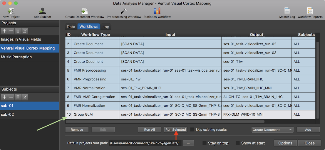
After clicking the OK button, the specified Group GLM workflow appears in the Worfklows tab (see row 10 in the Workflows table shown above). To execute it, the Run Selected button can be clicked after selecting the GLM workflow in the table.
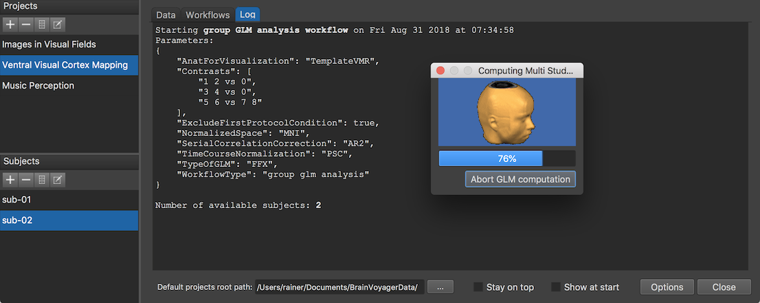
The Log tab will report the progress of the workflow (see screenshot above) involving in this case the creation of a multi-subject design matrix and integration of 6 VTC documents (3 runs of 2 subjects) in the GLM calculation. After finishing the workflow, an entry is added in the group-level data table of the Data tab (s. snapshot below). The Name of Group-Level Data column shows that the generic name of the created GLM document (here "FFX-GLM_WFID-10_MNI") is based on the GLM type (FFX-GLM),. The "WFID" substring with value "10" refers to the ID (usually row number) in the workflow table in order to uniquely identify the GLM in case that multiple workflows with slightly different settings are defined and executed, and the last substring identifies the normalized space (here "MNI") of the data. The Type column explicitly identifies the GLM type, the used time course normalization and serial correlation correction method.
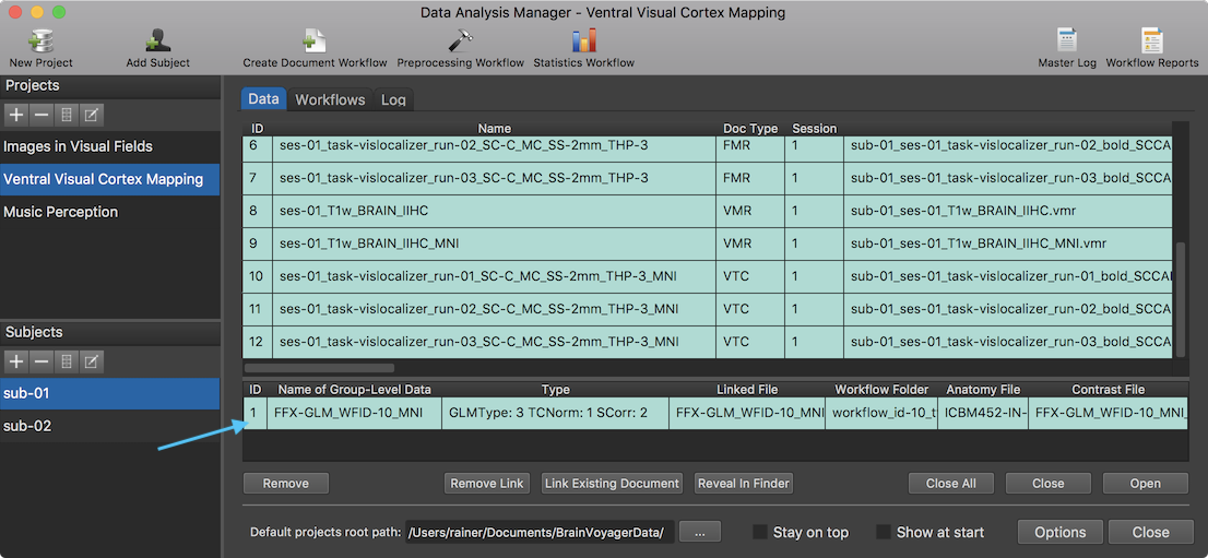
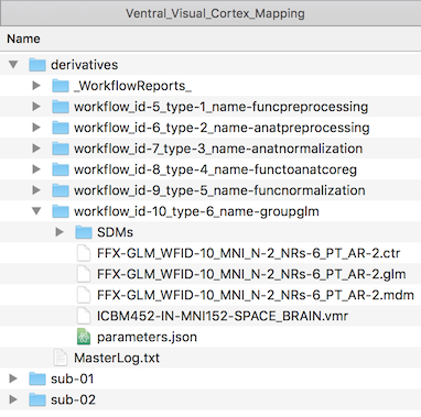
The Linked File column contains the name of the GLM file as stored on disk; similarly, the Anatomy File column contains the name of the VMR document that is used to overlay the statistical contrast maps; the contrasts that should be calculated using the beta estimates from the GLM are stored in the .CTR file displayed in the Contrast File column. These referenced files are stored on disk in the workflow folder (see screenshot below) inside the "derivatives" folder (or in the "GroupAnalyses" folder within the respective project root folder when not using BIDS mode). After selecting the respective entry in the group-level data table in the Data tab, the workflow folder can be displayed in a standard file browser by clicking the Reveal In Explorer (Reveal in Finder on Mac) button. The subfolder "SDMs" contains the created design matrix files for each run of each subject.
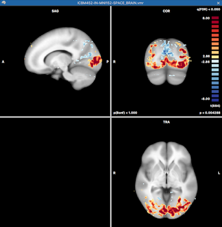
The results of the GLM (overall F test) are shown overlaid on the chosen anatomical VMR document in the standard BrainVoyager multi-document area. Since the template option had been chosen (default) for MNI normalized data, the standard MNI template data set ("ICBM452-IN-MNI152-SPACE_BRAIN.vmr") is used as the underlying document for the statistical map data (see snapshot below).
Furthermore, all specified contrasts (3 in the example, see above) are readily available when opening the standard Overlay GLM Contrasts dialog. The prepared contrasts file can also be explicitly loaded using the Load .CTR button. The screenshot below shows the third of the three defiend contrasts. By turning on the Overlay all contrasts option (see green rectangle) before clicking on OK all contrast maps will be calculated and made available for selection in the Volume Maps dialog.
The screenshot below shows the Volume Maps dialog on the right side with the three calculated contrast maps. The last (here third) contrast map has been selected as default but any other contrast map can be selected as usual. Furthermore other map display parameters, such as threshold values and colors, can be adjusted in the dialog.
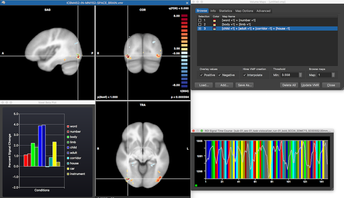
The left side shows the VMR document with the selected volume map as thresholded overlay corresponding to the evaluation of contrast 3. The Voxel Beta Plot dialog shows beta values retrieved from the location of the mouse position hovering over the VMR document view, which has been put at the location of the white cross. Furthermore, the ROI Signal Time Course dialog shows the time course of the selected cluster for the first run of the first subject and any other run can be selected using the standard options in the (expanded) dialog.