Turbo-BrainVoyager v3.2

The Stimulation Protocol Dialog

Using the Stimulation Protocol dialog, you can define the conditions for your experiment and the intervals during which the conditions occur. A protocol file forms the basis for the statistical analysis but is also important for visualization purposes.

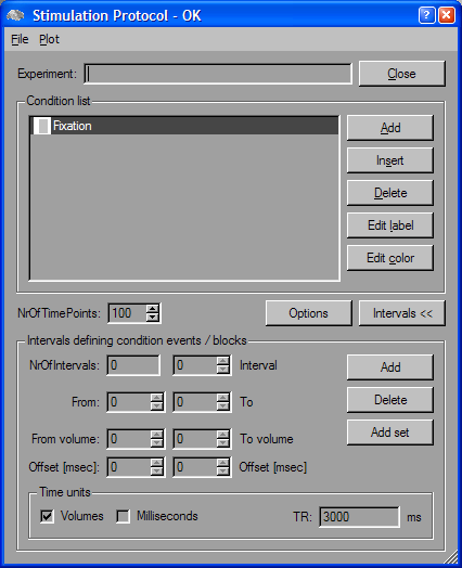
Click the Stimulation Protocol item in the Analysis menu to invoke the Stimulation Protocol dialog. You can name the paradigm in the Experiment field as desired.

To define a new condition, click the Add button on the right side of the Condition list. You will see "<untitled>" in the Condition list. Select the "<untitled>" entry and then click the Edit Label button. The appearing text dialog allows you to change the name of the new condition as desired. Enter a name and then press the <RETURN> button.

The most important information you have to provide next are the intervals during which the defined condition is defined. You can enter the intervals in specific fields, which appear after clicking the "Intervals >>" button:

In the "Intervals defining condition events / blocks" field, you can now define the intervals for the condition currently selected in the "Condition list". There are two ways to specify a protocol:

a) Specifying the intervals numerically, i.e. for each interval of a condition, the time point when an interval begins and the time point when the interval ends has to be entered.

b) Using a graphical procedure based on a segmented visual representation of time.

Numerical definition of condition intervals

The numerical specification of intervals is a very flexible approach, which works also in cases when the intervals of conditions have different length (duration). To define a new interval, make sure that the respective condition is selected in the "Condition list" (i.e. "Fixation" in the snapshot above) and then click the "Add" button in the "Intervals defining events / blocks" field.

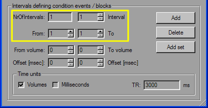
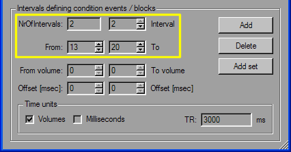
As a result, the NrOfIntervals field now shows that we have "1" interval defined for the currently selected condition. If more than one intervals have been defined, the Interval field can be used to browse them. At present, this field shows also "1" because only one interval has been defined. As default, the begin and end point of the interval are set to "1" as shown in the From and To fields. You may now change these values. As an example, change the To field to "8". You can define additional intervals for this condition by pressing the Add button. Define a second interval and set the From value to "13" and the To value to "20". Now the NrOfIntervals field indicates that there are two defined intervals for the current condition and you can select either one by changing the Interval field. In the snapshot below, the second interval is selected.

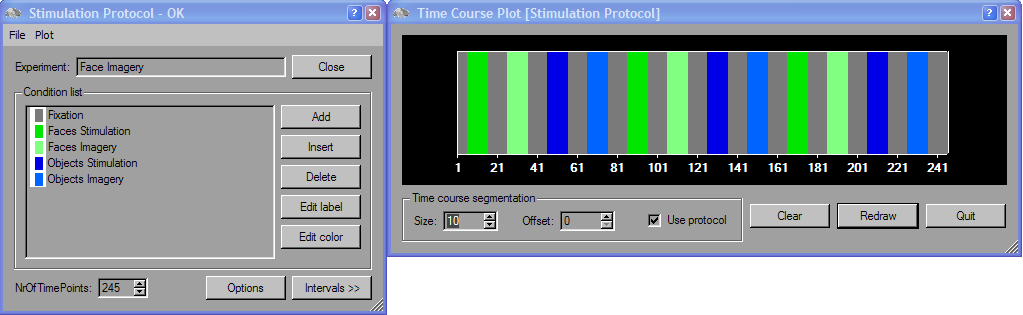
You can visualize the specified intervals in a graphical representation of the protocol. Click the Plot -> Time course plot window item in the dialog's local menu to call the Time Course Plot [Stimulation Protocol] dialog. As default, this dialog shows a time course with 100 data points corresponding to the NrOfTimePoints entry in the middle of the Stimulation Protocol dialog. You may change this value, which is, however, not necessary because it will expand automatically if you define intervals stretching beyond 100 time points. In the Time Course Plot dialog, you should see colored bars visualizing the conditions and intervals defined so far. Each condition gets a default color, which is grey for the first defined condition because the first condition defined is often a "Rest", "Baseline" or "Fixation" condition. You can change the color used for a condition by clicking the Edit Color button next to the Condition List. If you do not see the bars (see below), make sure that the Use Protocol option in the Time Course Plot window is turned on.

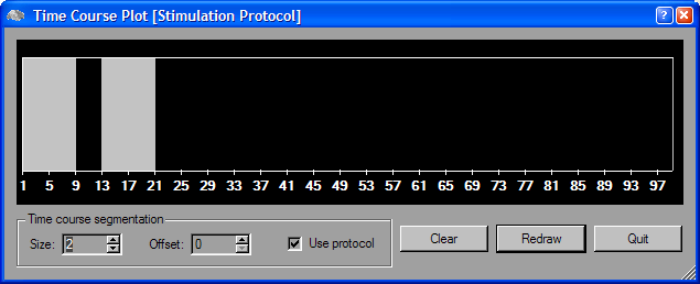
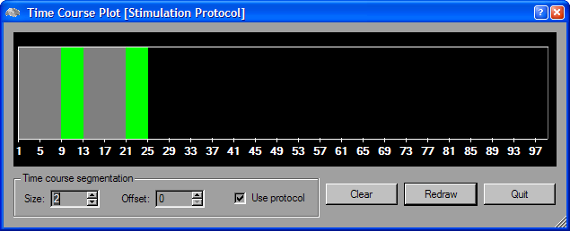
In the same way as described for the first condition, you can add additional ones. To add a condition, click the Add button next to the condition list in the upper half of the dialog. Change the condition's name using the Edit Label button. While the new condition is selected in the Condition List, click the Add button in the Intervals defining events / blocks field to define the first interval for that condition. Enter the value "9" in the From field and the value "12" in the To field, which fills the period left blank by the first condition. Add another interval by clicking the Add button and enter the value "21" in the From and "24" in the To field. The protocol defined so far should look like in the snapshot below (the condition colors have been changed using the Edit Color button):

In the same way, you can add further conditions and intervals for the conditions. Note that the numerical technique allows you to define any length ("duration") for an interval and presents, thus, a very flexible way to define protocols.

Graphical definition of condition intervals

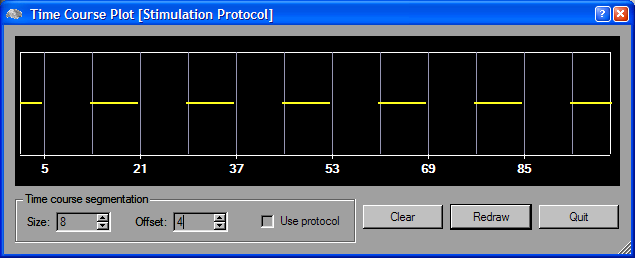
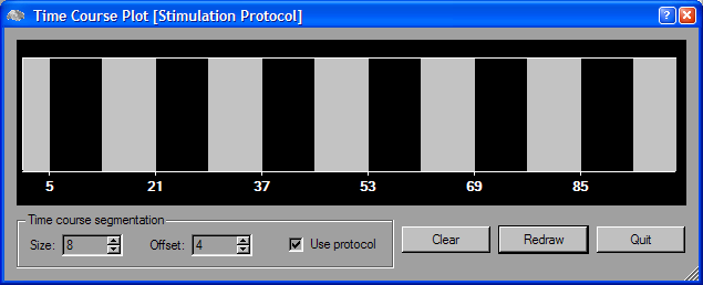
The graphical method works well with regularly spaced conditions, i.e. if you have stimulation periods of equal length (i.e. 8 blocks of condition 1, then 8 blocks of condition 2, then 8 blocks of condition 1 etc.). To get a graphical representation of the protocol, click the Plot -> Time Course Plot Window item in the dialog's local menu to call the Time Course Plot [Stimulation Protocol] dialog. As default, this dialog shows a time course with 100 data points corresponding to the NrOfTimePoints entry in the middle of the "Stimulation Protocol" dialog. You may change this value by using the spin buttons or by directly entering a new value. At the beginning, this dialog shows a series of vertical lines located at increments of 10 time points. When the segmentation lines are not visible, unmark the check-box Use Protocol to reveal them.

Click the spin buttons of the Size field to change the separation of the vertical segmentation lines (here the value "8" is used). Although many protocols have a regular spacing, the beginning and ending part of a protocol often have a different length. You do not have to care about the ending part, but for the beginning segment, you can enter a specific length by changing the Offset field. If you change the Size and Offset fields, the program immediately updates the segmentation lines accordingly.

After setting the Size and Offset value, click with the left mouse button in all segments belonging to the condition currently selected in the Condition List (i.e. "Fixation"). As a result, the selected segments will be marked with horizontal yellow lines as shown below:

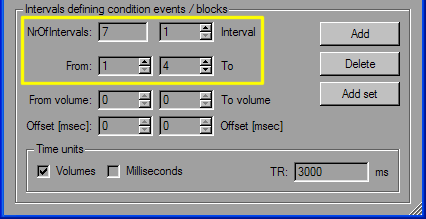
To convert the performed graphical specification into a numerical representation, click the Add Set button in the Intervals defining events / blocks field of the main dialog. The started process reads the begin and end points of the horizontal lines and stores them as a list of intervals for the condition currently selected in the Condition List (i.e. "Fixation"). You can check the result by looking in the respective fields in the lower part of the dialog (see yellow box in the snapshot below). The NrOfIntervals entry now has a value of "7" corresponding exactly to the number of horizontal line segments selected with the mouse in the Time Course Plot dialog. The Interval field currently shows the first ("1") defined interval which is from "1", as shown in the From field, to "4", as shown in the To field. This corresponds to the first horizontal line, which is only "4" time points long because this value was specified in the Offset field. You can now select any of the seven defined intervals by using the spin box of the Interval field. If you want to adjust an interval, you can do this directly by changing the From and To fields.

The definition of the intervals is also reflected in the Time Course Plot, which now turns on the Use Protocol option and shows seven vertical bars defining the thus far defined protocol.

The condition gets a default color; the first condition is colored grey because it usually defines a "Rest", "Baseline" or "Fixation" condition. You can change the default color by clicking the Edit Color button next to the Condition List.

In the described way, you can add additional conditions and define the respective intervals graphically or numerically. You can save your completed protocol using the Save Stimulation Protocol item in the dialog's File menu. A created protocol can then be specified in the TBV File dialog or directly in a TBV file.

Note. It is highly recommended to always define a rest condition as the first condition since other functions in TBV assume this and extra effort needs to be done if another condition (or no condition) is defined as the baseline. The setup of the design matrix for whole-brain and ROI GLM calculations, for example, treats the first condition of a protocol in a specific way by not modeling it explicitly as a predictor of interest but implicitly as a confound predictor (the "constant" predictor having value 1 at each modeled time point).

Note. The consistency of your protocol definitions are constantly checked in the background. The result of this consistency check is shown in the title bar of the Stimulation Protocol dialog. If "OK" appears, your protocol is fine. If, however, "NOT OK" is shown, your protocol contains overlapping condition intervals and you must change the protocol.

Note. You can also define a protocol in "millisecond" resolution, which might be necessary for some event-related paradigms. To define a protocol in millisecond resolution, click the Milliseconds option in the Time units field of the Stimulation Protocol dialog. You can then define your intervals numerically as described above. The only difference to the previous description is that you specify the begin and end of intervals using milliseconds instead of time points (volumes). Instead of entering absolute (large) numbers for the begin and end of an interval, you can also use the From volume and To volume fields together with the respective Offset [msec] fields. This allows to define the begin or end of an interval in milliseconds relative to a time point (volume). If, for example, a condition begins 300 milliseconds after the 12th volume (TR), you may enter "12" in the From volume field and "300" in the respective Offset [msec] field. From these two values the program computes an absolute value in milliseconds, which is shown in the From field. When using this approach, make sure that the TR value has been entered correctly since this value is used to compute the absolute value, i.e. AbsoluteValue[msec] = Volume[number] x TR[msec] + Offset[msec].