Turbo-BrainVoyager v3.2

Running Example Data Sets

The Turbo-BrainVoyager Installer CD includes two example data sets that can be used to practice working with the various features of the software. After installation, the data sets are stored in the "(My )Documents/TBVData" folder (if not deselected). The installers on our web site do not include the sample data sets but you can get them there as a separate download. If you download the exercise data, extract the .zip files in the "Documents/TBVData" folder. Since the provided .TBV files support relative path names, it is, however, not critical where the sample data will be installed.

TBV will run with a sample data set in the same way as during a real scanning session (it doesn't know the difference). During scanning, TBV usually reads the next data volume as soon as it becomes available. Note that in case of running sample data, the complete series of functional volume data is already available on disk and, thus, the analysis will run likely much faster than in the real scanning situation. In order to more realistically simulate the experience during a real scanning session, one may want to set theForceTRDelay option to "true" in the Statistics tab of the TBV Settings dialog. You may also press the R key during a running analysis in order to switch between simulated true scanning speed and the maximally possible speed.

"Faces Houses" Data

This data set allows to localize in real-time the fusiform face area (FFA) and the parahippocampal place area (PPA). Besides rest blocks, 2 blocks with images of faces and 2 blocks with images of houses/places are shown. To analyze this sample data set, select the TBV file "NK_FFA_PPA_TAL-1.tbv" in the "TBV_FacesHouses" folder using the Set TBV File item in the File menu. Then press the red Record button to start real-time analysis. If you want to speed up processing, press the R key. The program always launches in multi-slice view. To become familar with TBV, it is recommended to perform the following tasks:

Select regions-of-interest (ROIs) by dragging the mouse over any section of a slice.
Click CTRL-R to switch between ROIs visualized as rectangles or as marked voxels.
Add a new ROI by dragging a region while holding down the SHIFT key.
Replace the content of a Time Course Window by first clicking it to make it the active one followed by a dragging operation.
Change the threshold of the displayed maps using the Threshold spin box in the lower right corner of the program window.
Press CTRL-B to hide or show the beta plot section on the right side of Time Course Windows.
If the analysis of a run has been completed, right-click a time course window and select ROI GLM in the context menu.
Zoom into a slice by clicking on it while holding down the ALT key. ALT-click again to go back to Multi-Slice View.
Switch to the available Brain Views using the icons below the main window.
Switch to Volume View to inspect how the plots change dynamically in the Event-Related Averaging Plot.

You will also find a recorded animation on our web site demonstrating these and other possibilities of Turbo-BrainVoyager. Furthermore, the TBV installer puts a more detailed tutorial document "TBV_Exercise1_FacesAndHouses.pdf" in the "(My )Documents/TBVData/TBV_FacesHouses" folder.

"Attention BCI" Data

Attention BCI Stimulus

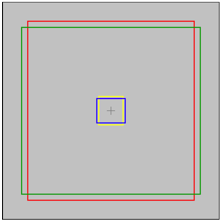
This data set consists of several runs. The subject is asked to attend either a local or a global rectangle displayed on the screen (see snapshot above). The first run is used to train a classifier to associate the brain activity patterns evoked during the two tasks with the respective condition. When the subject performs the attention task in subsequent runs, the trained classifier is used to predict the condition from the evoked brain patterns. To analyze the first run used to train the classifier, select the TBV file "ATTBCI_01_trainig.tbv" in the "TBV_SVMClassifier" folder using the Set TBV File item in the File menu.

SVM Training

It is recommended to perform the following tasks:

Run through the data in as-fast-as-possible mode (this mode is set as default in the TBV file for this run).
During real-time analysis, inspect any region you desire. Note that it is difficult to find regions that clearly discriminate between the two conditions "small" (attention to small rectangle) and "large" (attention to large rectangle).
When the analysis of the run has been completed, define a ROI for training. Since this ROI should include almost all grey matter voxels in the back of the brain, lower the threshold of the displayed maps, e.g. to a value of "2.0" and turn on the contrast "small vs resting" and "large vs resting" in both directions (i.e. mark all 4 option boxes for these two contrasts).
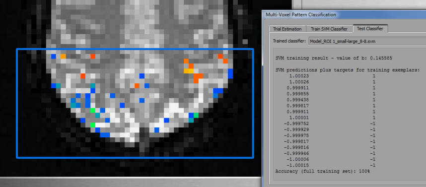
Increase the value of the MultiSliceROIs spin box to 18. Now drag a rectangle at a slice in the middle of the brain in such a way that it encompasses most of the posterior cortex (see snapshot above showing a specified ROI in both rectangle and marked voxels view).
Enter the Multi-Voxel Pattern Classification dialog and prepare the training as described in the SVM Training documentation (see also snapshot above).
After training the classifier, you may inspect the distributed weights of the SVM classifier since the original map will be replaced by a map of SVM weights; increase the threshold to see where high values are located (see snapshot below).

SVM Weights

To analyze the second run - used to test the trained classifier - select the TBV file "ATTBCI_02_testing_1.tbv" in the "TBV_SVMClassifier" folder using the Set TBV File item in the File menu. Note that in the context of classifier applications, it is most convenient to set the WatchFolder for all runs of one scanning session to the same output directory. In this case it is easy to find the classifier output data from previous runs when preparing classifier testing. For the sample data used, the target folder has been set to "ATTBCI_TBV_analysis" (within the "TBV_SVMClassifier" folder) in the TBV files of all runs.

After selecting the TBV file for the first test run, perform the following tasks:

Open the Real-Time SVM Classification dialog.
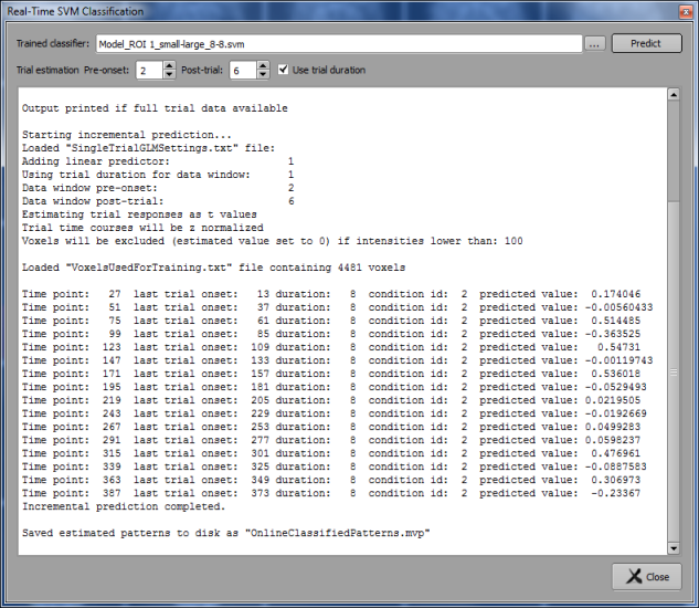
Use the Browse button next to the Trained classifier text box and select the SVM file of the classifier trained with the data of the previous run (e.g. "Model_ROI 1_small-large_8-8.svm", see also snapshot below).
Click the Predict button. The program now waits for data to analyze.
Click the Record button to start data analysis.
Observe the incremental predictions of the classifier. Note that the protocol of the test run(s) do not encode the condition, i.e. it does not encode the task (all task epochs are coded with the same condition labelled as "2" in the classifier output). In order to evaluate the classifier performance, the subject was asked to alternate the "small" and "large" attention tasks.
Are all task epochs classified correctly? In the snapshot below, the accuracy is 94% - Do you spot the one trial predicted wrongly?

SVM Weights

There are two more runs that can be used for testing in the same way as described above. Note also that you can use the data from more than one run for training, i.e. you can use the data from the first two runs for training and then test the classifier on the two additional runs. The TBV installer puts a more detailed tutorial document "TBV_Exercise2_AttentionBCI.pdf" in the "(My )Documents/TBVData/TBV_SVMClassifier" folder

SVM Weights

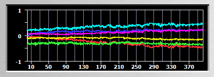
Note. You may be surprised to see non-zero motion parameters at the begin of a run in the Motion Correction Window when analyzing the test runs (see snapshot above). This does not reflect real motion of the subject at the begin of the scan (the subject actually does not move much) but happens because subsequent runs use the first (training) run as their target for motion correction. While the subject itself does not move much as indicated by the motion parameters, there are small incremental motion effects across runs (e.g. due to scanner gradient heating) and these effects will be corrected by across-run motion correction.