Turbo-BrainVoyager v3.2

Real-Time SVM Classification

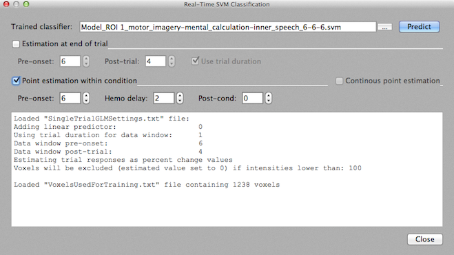
For BCI applications it is necessary that a classifier can be used incrementally, i.e. on a trial by trial or time point by time point basis: As soon as enough data points are available to estimate response values for the voxels used during training, a real-time classifier provides a "guess" (prediction) about the class to which the actual distributed activation pattern likely belongs. The Real-Time SVM Classification dialog (see snapshot below) allows to run such an online SVM classifier after an appropriate training phase. The dialog can be invoked using the Real-Time SVM Classification item in the Analysis menu. The previously trained SVM classifier needs to be specified using the "..." browse button next to the Trained classifier text box. Note that you can use the output value(s) of a running classifier as a neurofeedback signal; for details read the topic Classifier Output Feedback and the SVM Access plugin functions.

The dialog offers two prediction modes:

Trial-by-trial prediction. Prediction is generated once at end of a trial.
TR-by-TR prediction within condition. Prediction is generated at each time point within (shifted) condition phases.
In a future version, continuous TR-by-TR prediction will be added. Prediction will then be generated at each time point without using a protocol.

In order to know how trials have been estimated during training, the program looks for a file called "SingleTrialGLMSettings.txt" containing the settings used during training. This file is automatically saved when estimating trial responses for the training data. If the data of the current run resides in a different target folder than the data used during training, you should manually copy that file into the current folder, otherwise default settings will be used (that may or may not reflect the settings specified during training correctly). The settings that will be used for trial estimation are printed in the Log pane (see snapshot above).

The online classification also needs to use the same voxels for extracting trial responses as used during training. In order to get this information, the program looks for a file called "VoxelsUsedForTraining.txt" containing a list of the coordinates of the voxels used during training. This file is automatically saved when the training data is created prior to training for a selected ROI. In addition to this file, a standard .ROI file "VoxelsUsedForTraining.roi" is available allowing to load the ROI into the main window using the Analysis > Load .ROI Definition File menu. If the data of the current run resides in a different target folder than the data used during training, you need to manually copy the "VoxelsUsedForTraining.txt" file into the current folder, otherwise the classifier will not work. The Log pane will show whether the file was found and how many voxels are defined in that file (see snapshot above).

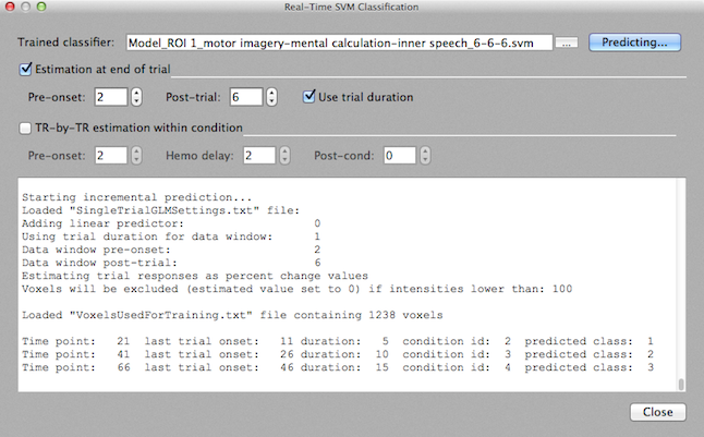
When all necessary information is available, a click on the Predict button starts the online classifier. In order to signal that the classifier is enabled, the button text changes to "Predicting..." and the message "Starting incremental prediction..." is printed in the Log pane. Typically the Predict button is clicked after having started standard real-time processing, i.e. after clicking the red Record button in the main program window to process a new run after SVM training. The classifier can be turned off any time by clicking the Predict button again; the classifier also stops working if the currently processed run ends; if the classifier stops, the text of the Predict button will change back to "Predict" from "Predicting..." and the Log pane will print the message "Incremental prediction completed."

Trial-by-trial prediction

This approach was introduced in version 3.0 of TBV. The running classifier uses the current protocol to retrieve information of the onset and duration of trials. It requires that there are baseline phases between defined main condition intervals and that the baseline phases are not used as a separate class during training, i.e. 2 or more main conditions should be used as class labels. Note that the protocol used for a test run needs not to define specific conditions, i.e. next to the baseline condition, 1 main condition is sufficient (e.g. "unknown task") to know the time periods when the subject is asked to perform a task that needs to be classified (see also below).

The trial-by-trial prediction approach performs a trial estimation step as soon as enough data points are available for the currently processed trial. Then at each voxel in the ROI a single-trial GLM is fitted to the data in a time window that needs to include a baseline period before the protocol condition onset and a baseline period after condition offset. A design matrix is then constructed that contains a constant predictor (confound to estimate the baseline level) and one predictor of interest modelling the voxel's response to the current condition using the standard two-gamma hemodynamic impulse response function. If included during training, a linear predictor will be added as a second confound; this is not recommended if the time courses have been detrended using post-processing.

The estimated single-trial task beta value is then used as the voxel's response contributing to the spatial distributed pattern for the current trial that is submitted as a test pattern to the classifier. Note that there are several options to normalize the estimated beta (e.g. as percent change values or t values) and the program will automatically perform the same normalization as used during training based on the "SingleTrialGLMSettings.txt" file. In order to use this prediction option, check the Prediction at end of trial option. The displayed Pre-onset and Post-trial (or Post-onset) values will be automatically set based on the retrieved settings from the previous learning phase and it is not recommended to change these values.

Information about the processed trial as well as the output value predicted by the classifier is printed within one line in the Log pane. The first line after the "Starting incremental prediction" text shown above, for example, indicates that the first trial is processed at time point 17 since at this point the data window for the trial that started at time point 9 is complete (with respect to the used trial duration and post-trial settings). The printed line also shows the duration of that trial (5 time points) and the condition number (id) of the corresponding condition in the protocol (2). The final value is the predicted class label (which is "1" for the first trial shown above). In this example, the protocol assigns the trials to different conditions since the subject was instructed to perform a specific mental task. Note, however, that the classifier would also work fine in case that the protocol would define only one condition (e.g. "unknown task") since the classifier only uses the onset and duration information from the protocol but not any information about the condition to which the trial belongs. In a brain reading paradigm in which the subject freely may decide which task to perform, the protocol will not contain any specific condition information and the condition id will be not informative. In case that the subject performs mental tasks in a prescribed order (as in the displayed example), a comparison of the condition id with the predicted class can be used to assess the accuracy (generalization performance) achieved by the classifier for the new data set.

TR-by-TR prediction within condition

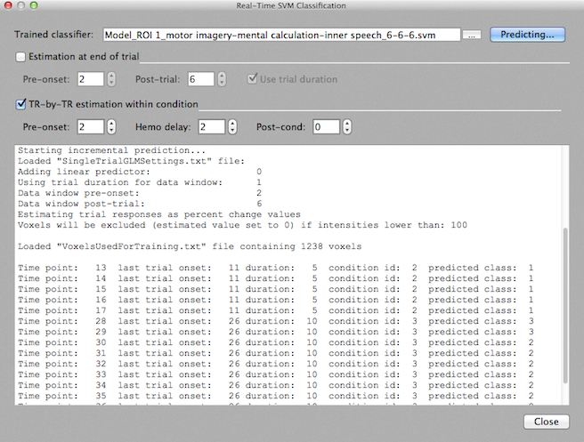
As in the trial prediction approach, the running classifier in this mode (added in version 3.2) uses the current protocol to retrieve information of the onset and duration of trials. The TR-by-TR within condition approach also requires that there are baseline phases between defined main condition intervals and that the baseline phases are not used as a separate class during training (e.g. only 2 or more main conditions should be used as class labels). The difference to the trial-by-trial prediction approach is that voxel responses are not fitted only once at the end of a trial (i.e. after decay of the hemodynamic response) but for each (shifted) time point within defined main condition periods. Prediction values are, thus, produced as soon as a condition starts - except for a specified shift of data points with respect to condition onset in order to adjust for the hemodynamic delay. Since classification starts during an ongoing trial, the classification output of this approach can be used as input for moment-to-moment neurofeedback. You can use the Hemo delay spin box to set an appropriate shift value for your functional scan. If the TR is, for example 2 seconds, a shift value of 2 or 3 would be recommended (the BOLD signal is expected to start rising after 3-4 seconds). With a value of 2 for example, the first classifier output would be produced immediately when the data for the 3rd time point of the current condition would become available. Additional predictions will then be produced for subsequent time points until the condition ends plus the shift value; the number of sequentially predicted values depends on the duration of the current protocol condition interval. In case you want to extent predictions beyond the shifted condition duration, set the value of the Post-cond spin box accordingly (default value is 0).

In the same way as the trial-by-trial prediction approach, this approach uses a GLM at each included voxel to obtain a response estimation. The constructed design matrix, however, only contains a "stick" predictor for the currently processed time point, i.e. no 2-gamma function is used for trial estimation. Instead of a single-trial GLM a single-TR GLM is calculated for each time point within a (shifted) condition period. Each constructed design matrix contains a constant predictor (confound to estimate the baseline level) and one predictor of interest modelling the voxel's response at the current time point within the (shifted) condition interval. If included during training, a linear predictor will be added as a second confound predictor. The estimated single-point beta value is finally used as the voxel's response contributing to the spatial distributed pattern for the current trial that is submitted as a test pattern to the classifier. As in other approaches there are several options to normalize the estimated betas (e.g. as percent change values or t values) and the program will automatically perform the same normalization as used during training based on the "SingleTrialGLMSettings.txt" file. For this approach it is recommended to use the "percent change beta" normalization approach. In order to use this prediction option, check the TR-by-TR prediction within condition option. The displayed Pre-onset value will be automatically set based on the retrieved settings from the previous learning phase but the value for the Hemo-delay spin box (number of shifted data points) and optionally the value for the Post-cond spin box need to be set by the user.

Information about the processed time point as well as the output value predicted by the classifier is printed within one line in the Log pane. The first line starting with "Time point:" above, for example, indicates that the first time point is processed at time point 13 since at this point the shifted hemodynamic response for the first time point (11) of the condition interval is available (11 + 2 = 13). The printed line also shows the duration of that trial (5 time points) and the condition number (id) of the corresponding condition in the protocol (2). The final value is the predicted class label (which is "1" for the first trial shown above). The second line shows the output for time point 14, i.e. the next time point for the current condition interval. The last output for the first trial is produced at time point 17 since the duration of the current condition interval is 5 time points. If there would be a post-condition value greater than 0, additional values would be produced, i.e. during the decay of the BOLD response. The sixth line marks the begin of the output for the second trial of this run. The condition interval starts at time point 26 and the first predicted output is, thus, obtained as soon as the data for the 28th time point is available. Since the corresponding condition interval has a duration of 10 time points, 10 output lines are produced for this trial. In this way, time points within each subsequent trial will be incrementally processed. Note that classifier output is generated as soon as possible and can be, thus, used for BCI and neurofeedback applications.

Notes

A continuous TR-by-TR prediction approach will be added in a future release (scheduled for TBV 3.4).

The Real-Time Classification dialog does not block other windows. It is, thus, possible to inspect time courses, switch to different viewing modes, change the t threshold of GLM contrast maps and so on while the classifier is working. There is also no conflict of the ROI used by the classifier with other selected ROIs since the classifier ROI is stored separately from the ROIs used in the main window.

At the end of a run, all estimated multi-voxel patterns are stored in a .MVP file with the name "OnlineClassifiedPatterns.mvp"; you may select this file in the Training/test data field in the Train SVM Classifier tab of the Multi-Voxel Pattern Classification dialog and visualize the patterns by clicking the Plot button on the right side of the selected .mvp file.