Turbo-BrainVoyager v4.4

GLM Confound Settings

Linear and non-linear drifts in voxel and mean ROI time courses have a negative effect on (incremental) statistical analysis leading to low t-values for effects of interest and to suboptimal calculations for applications such as neurofeedback. In order to remove such drifts from time courses during moment-to-moment real-time processing, it is recommended to add linear trend and non-linear drift predictors to the GLM design matrix. Enabling motion correction usually also reduces drifts in time courses; furthermore, adding incrementally (volume-by-volume) calculated motion detection parameters to the GLM design matrix may also remove llow-frequency drifts as well as other higher-frequency noise sources. Adding confound predictors (see below) model and thereby remove some noise sources from voxel time courses improving visualization of effects of interest in statistical maps.

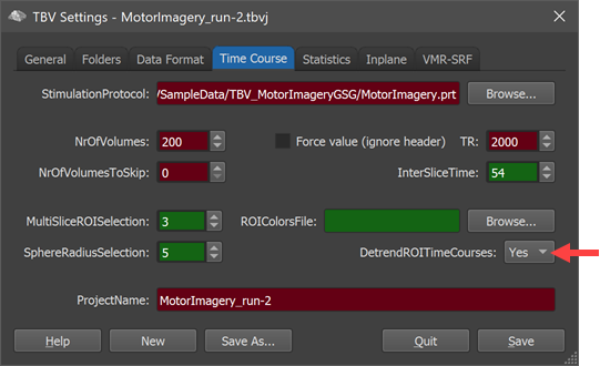
Estimated drifts can also be used to “detrend” ROI time courses by subtracting their effect from the original time course. Detrending of time courses can be turned on or off using the DetrendROITimeCourses option (see screenshot above) that can be set to 'Yes' (default) or ‘No’ in the Time Course tab of the TBV Settings dialog. Note that detrending can also be turned on and off during real-time analysis (or after reloading analyzed data) by pressing the D key or by using the corresponding option in the View menu allowing to assess the effect of confound predictors as demonstrated below. Since ROI time courses are also used as input for subsequent calculations such as neurofeedback, one should keep detrending enabled (or disabled) throughout an entire neurofeedback run. Note that since TBV 4.2 time courses are detrended and converted into percent signal change (PSC) values for easier interpretation of the amplitude of signal fluctuations. The PSC values of detrended time courses are also used directly as input for neurofeedback calculations.

Drift Predictors

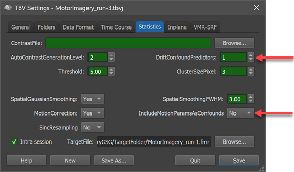
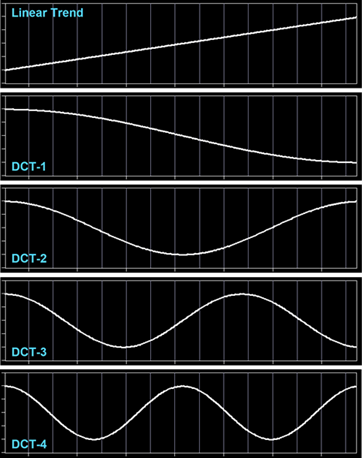
In order to add linear and non-linear drift predictors to the deisgn matrix, set the DriftConfoundPredictors value in the Statistics tab of the TBV Settings dialog (see upper red arrow in the screenshot above). Setting the value to '0' does not add any drift-related confound predictors (a 'Constant' predictor is always added). Setting the value to '1' adds a linear confound predictor (see top plot in figure below). Setting the value to '2' adds a linear confound predictor plus two low-frequency drift predictors generated from a discrete cosine transfrom (DCT) basis set (see image below). Increasing the value further will add additional DCT drift confound predictors up to a maximum of 6; the figure below shows the added confound predictors when entering value 4 in the the DriftConfoundPredictors field.

Note that these predictors are defined over the whole expected time course leading to highly correlated predictors at the begin of real-time processing when only a few (less than ca. 15%) data points are available. This may lead to a (close to) singular matrix when fitting the GLM to obtain beta values, especially when using incremental GLM calculations. In order to avoid unstable beta estimates, the program uses a full GLM implementation for (detrended) ROI time courses; for map calculations (i.e. for each voxel's time course), a full GLM is employed at every 25th time point up to time point 100. Between these full-GLM 'anchor' points and after time point 100, incremental recursive least squares (RLS) GLM calculations are used. With this approach, stability is maximized with only a limited dependence on more time-consuming full GLM calculations. For further information see section ‘Comparison and Advice’ below.

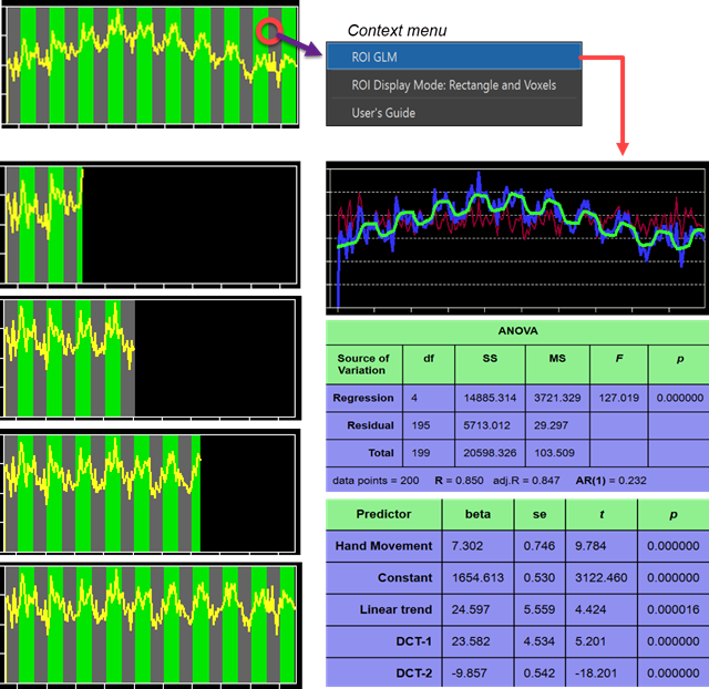
The figure above shows how confound predictors estimate and remove a non-linear drift in a ROI time course (left upper panel). The other panels on the left side show that drifts are removed successfully throughout real-time processing as indicated by the stationary (detrended) time courses. The right side of the figure above shows detailed results of the GLM fitted to the full time course data. This information can be invoked by right-clicking a ROI time course and then clicking the ROI GLM item in the appearing context menu as indicated above; note that the ROI GLM feature is only enabled at the end of a real-time run or after reloading previously analyzed data. In the example above a DCT-2 confound model has been specified, which is sufficiently complex to remove linear and most non-linear low-frequency drifts typically observed in fMRI data. Adding more confound predictors may help in some rare cases but is not recommended in order to avoid close-to-singular matrices (see section ‘Comparison and Advice’). Since TBV 4.2, confound predictors are added to ROI time course GLM design matrices over time with a more sophisticated scheme in order to ensure optimal detrending results. For detais, see topic Detrending Predictors Timing.

Motion Predictors

Since TBV 4.0 it is also possible to incrementally add the motion parameters as confound predictors to the GLM design matrix, which has been proven beneficial in offline fMRI analyais. To enable this feature, the IncludeMotionParamsAsConfounds option in the Statistics tab of the TBV Settings dialog needs to be set to 'Yes'. As soon as the 6 motion parameters (3 translations, 3 rotations) have been estimated for a new volume, the values are added to 6 motion confound predictors respectively in the incrementally growing design matrix before new beta weights are estimated.

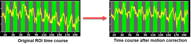
Note that motion correction itself, i.e. without putting the motion parameters in the design matrix, reduces drifts to some extent since drifts are partially caused by image displacement over time. The screenshot above shows on the left side an unprocessed time course with a moderate drift and on the right side the time couse when performing online motion correction. To produce the left panel, motion correction has been turned off by setting the MotionCorrection option in the Statistics tab to 'No' since motion correction is enabled as default because of its importance. The panel on the right side has been generated with motion correction enabled using the same ROI as before; for both panels, no detrending (no confound predictors except the constant) were added to the time course GLM design matrix.

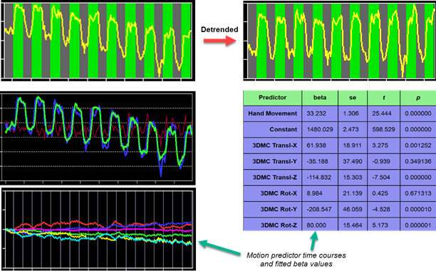
While motion correction reduces drifts by re-aligning incoming volumes to the first volume of a run (or to a volume in a previosu run), drifts are usually not completely removed from time courses. Using detected motion parameters as confound predictors is one possibility to remove additional drifts and noise from voxel time courses. The screenshot above shows a time course exhibiting a linear trend despite motion correction (upper left panel) and the result of detrending using the 6 motion predictors as confounds (upper right panel). Although no linear trend predictor was used, the motion parameters successfully removed the linear trend.

Comparison and Advice

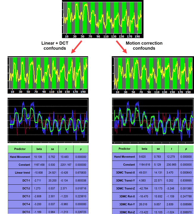
The figure below shows an example comparing a DCT-5 confound model (including a linear trend) with a motion predictors confound model. Below the two detrended time courses, the GLM model fit to the original data is graphically visualized followed by the numerical GLM table with the respective model predictors together with associated statistical values. As can be seen, each approach removes the non-linear trend in the original time course (top graph). Since the DCT model contains only smooth low-frequency basis functions (see above), the single hemodynamically convolved task predictor (hand movement) appears smooth and identical across all blocks of the experiment in the graphical fit display. Since the motion predictors contain also high-frequency variability, the task predictor shows that also some high-frequency fluctuations have been 'captured' by the motion predictors.

One might conclude that an even better result could be obtained by combining both confound predictor sets. As described above, adding many confound predictors to the design matrix may, however, lead to instabilities when fitting beta values at the begin of real-time analysis since predictors may be highly correlated. While TBV 4.0 increases stability by performing full-time course GLM calculations from time to time at the begin of analysis (every 25th time point up to time point 100) and always for detrending ROI time courses, it is not recommended to include both a large number of non-linear DCT predictors and motion parameters. If motion parameters are included as confounds, a linear trend or DCT-2 model (that also includies a linear trend) should be sufficient for most cases.

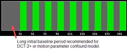
More generally, there is a tradeoff between quality of detrending and stability issues at the begin of real-time analysis. As a conservative approach that always leads to stable GLM fits, one would just add a linear trend predictor (value '1' in the DriftConfoundPredictors field) and no motion parameter confound predictors. While linear trends usually explain most of the low-frequency noise fluctuations, such a simple model does not remove curvilinear drifts. It is thus advised to use either a DCT model with values '2' in the DriftConfoundPredictors field or a linear trend plus motion predictors. While the program supports adding DCT and motion predictors, it will show a warning message with suggestions to turn off one of the two approaches. As another general recommendation it is suggested to use a long initial baseline period of at least 30 time points before the first task (e.g. neurofeedback) block in the experimental design as indicated in the image above when using more than a linear trend confound predictor. Since the DCT predictors are stretched across the whole expected data points, it is even more appropriate to consider a percentage of ca. 15% of expected volumes for the first baseline instead of a fixed number.

Incremental inclsusion of predictors. An important approach of TBV to get early and stable beta estimates is to start with a reduced design matrix adding predictors over time until the full GLM design matrix has been established. For main predictors this approach is employed since the first releases of TBV so that beta values can be calculated as soon as a predictor contains non-zero data. In an experiment with two main predictors, for example, the predictor for the first task would be added as soon as the first block is employed whilte the predictor for the second task is left out the design matrix until that task is performed the first time. When all main predictors are present also all confound predictors are added at once. Since TBV 4.2 the incremental addition of predictors is extended to confound predictors of ROI time courses as described in topic Detrending Predictors Timing.

Copyright © 2002 - 2024 Rainer Goebel. All rights reserved.