Turbo-BrainVoyager v4.4
Running the Real-Time ICA Plugin
As is the case for all TBV plugins, the real-time ICA plugin has two separate stages, a preparation stage and an execution stage. In the preparation stage, all general settings are to be defined by the user. These will characterize the entire TBV run and can not be changed dynamically during the execution stage. In the execution stage, the only required user interaction consists in the dynamic mask definition by which the user draws a rectangular box in the slice of interest to update the spatial reference used in the component selection. The box should include the brain region(s) of interest to be used as "seed" to retrieve the ICA component(s) of interest.
Preparation Stage
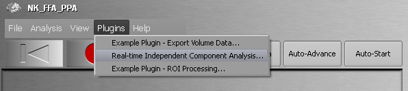
The plugin can be invoked from the Plugins menu. This immediately starts the preparation stage showing a Log window and a series of dialogs gathering choices from the user. TBV also prevents calling any other plugin until the running plugin is dismissed.
The real-time ICA plugin preparation includes the following steps:
1) Setting the first and last slice that will be included in the spatial ICA analysis:
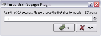

Note: At this stage, the plugin can not check how many slices will be part of the fMRI slab; it is therefore very important to provide correct values.
2) Setting the length of the moving time window (in time points):
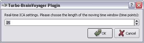
Note (1): This setting strictly depends on the application. In fact, if you, e. g., expect to find (and want to track over time) regions activated during blocks of, e. g., 15 time points (i.e. 30s if TR=2s), the suggested default of 25 points is a good choice since you can have both edges of the most expected activation response included most of the times, whereas windows shorter than 15 points may let you lose tracking of this pattern during the sustained phase of activation. In contrast, an ideal event-related response or change lasting 20s could require 10-15 points at TR of 2s. But keep in mind that the plugin doesn't use any model of the response shape and timing, therefore these considerations and thoughts can only provide an initial guess.
Note (2): This is also the parameter that most affect the performances. Using too many time points, in relation to the number of slices included, reduce the real-time performances. However, selecting 2-3 slices and setting a window of 25 points allows similar real-time performances as for a real-time (whole-brain) GLM on a standard computer.
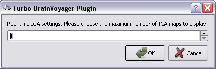
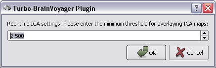
3) Setting the maximum number of ICA maps to display in real time and the threshold of the spatial ICA z score:
4) Step size for component map updating and saving:
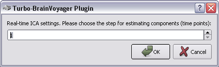
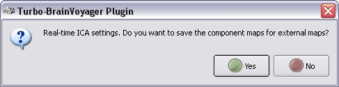
Note: Normally, components can be updated each time when a new fMRI volume becomes available, i. e. at each new time point. Sometimes, typically when longer time windows are used (substantially slowing down performance), the user may want to not update each time point but, e.g. after every 2 or 3 time points. Saving the component maps to disk for external use (e.g. neurofeedback is also optional and should be only included if necessary since it slows down the operation of the program.
Execution Stage
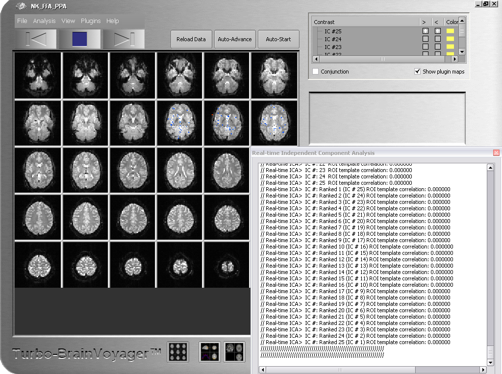
After the preparation stage, the plugin is in "stand-by" mode, waiting for TBV to start analysis providing preprocessed (e.g. motion corrected) functional data incrementally to the plugin. The Log window is also displayed with a summary of the choices made (see snapshot below). You may want to resize it to better view the presented text information.
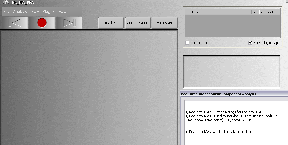
When the TBV analysis starts, the plugin starts. This also implies that the plugin maps (and not the GLM maps) will be shown as default. At any time during real-time analysis you may use the Show plugin maps option (see snapshot above) to toggle between ICA component maps and conventional GLM maps (since a GLM analysis is executed concurrently with the ICA analysis). Please note, however, that the actual computation of the ICA components only starts when enough time points have been acquired to fill up the first sliding window. From this moment onwards, components are extracted, ranked and displayed in real time with volume-by-volume acquisition as in any TBV session.
If the user does not interact with the program, he will see some maps overlaid on the included slices (see, e. g. the figure below where slices 10, 11 and 12 were included). However, you normally get random maps and therefore you may probably visualize just noise most of the time:
In order to make an effective selection, a dynamic mask should be drawn by the user. This can be easily done with the mouse, as shown below:
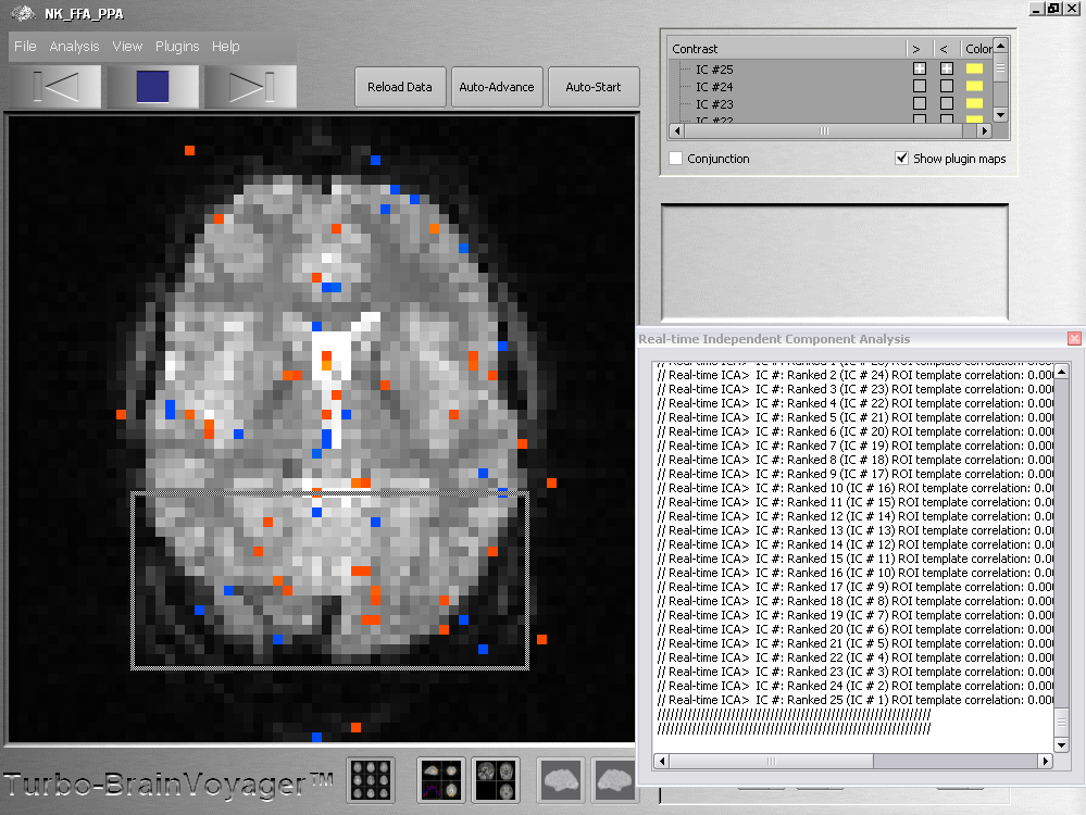
The consequence will be that from that moment on, a dynamic mask will be used by the plugin for selecting (and tracking over time) the ICA component (or components) whose maps maximally correlate (in space) with the mask. The tracking of this component will normally continue until either the user defines a new mask or until the activity pattern described by this component changes dramatically the layout with respect to the mask or in case that the component vanishes.
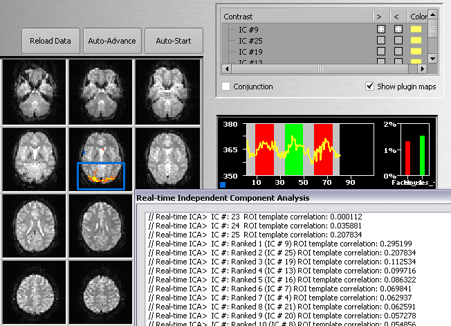
The following example shows a visual ICA component tracked over time and the dynamic mask that makes it possible. The contrast window shows the intrinsic ranking of the component, which, like the map, changes at each time point as a result of the selection. The Log window reports the spatial correlation coefficient of the template map obtained from the ROI mask and the (ranked) ICA maps. The time course is obtained from the region within the ROI.
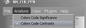
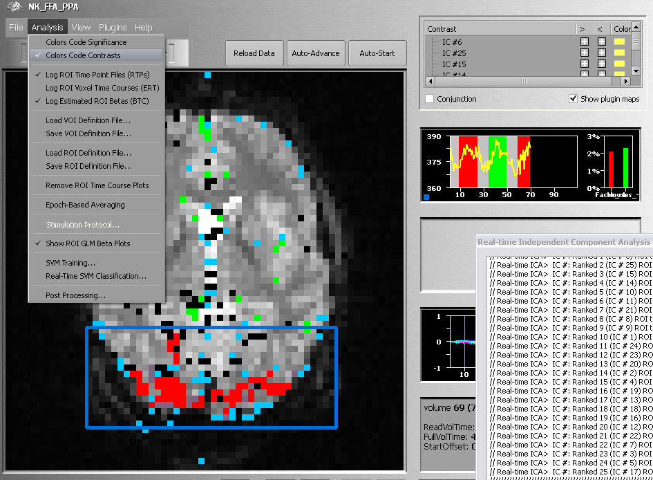
When choosing to display more than one ICA map at a time, it is more convenient to color code the different ICA maps separately rather than the z scores using the same color range. To switch color mode, select the Colors Code Contrasts item in the Analysis menu (the term "contrasts" identifies both GLM maps as well as plugin maps). The snapshot below shows the respective menu item; as a result, the different ICA maps are shown each in a different color.
Copyright © 2002 - 2024 Rainer Goebel. All rights reserved.