BrainVoyager v23.0

Group-Level ICA

Description and Purpose

Self-organizing group-level ICA (SogICA, Esposito et al., 2005) is a method to summarize individual ICA-decomposed data sets on a group level by clustering the independent components in the subject space. The linear correlation coefficient (computed between two spatial maps and/or two time-course of activity) is adopted as the similarity measure in the present version. The similarity measures are converted to Euclidean distances and these are used to fill a matrix of "distances". Based on the distance matrix, a supervised hierarchical clustering procedure is run, the supervising constraint consisting of accepting just one component per subject in each cluster formed by the hierarchical procedure. As a consequence, at high level of intersubject similarity the clusters are "closed" very rapidly but the lower the similarity (the more the subjects) the slower will be the search of valid "members" for the current cluster under formation and the lower the resulting intra-cluster similarity. The user can decide how many clusters to extract.

For the only purpose of "clustering" it is possible to:

Apply a user-specified threshold to each individual components (z-ICA scores) before estimating the spatial similarities (default: z=0, no threshold); this has the effect of setting to zero all component values below the threshold.
Apply a user-specified spatial mask via a mask file (*.msk) created on the native resolution of the components (normally 3x3x3 mm); this has the effect of including in the similarity analysis only component values from voxels included in the mask. Spatial masks can be applied in addition to component pre-thresholding according to point 1.
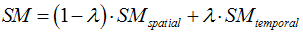
Inter-mix (at a user-specified degree) temporal similarity with spatial similarity using the individual component time-course of activity according to the following formula (default: lambda = 0, i.e. no temporal similarity used):

Group-level component maps can be generated (and visualized) in three different ways based on which specific parameter is estimated voxel-wise starting from each subjects' ICA z-value:

The mean ICA z-value is computed (fixed-effects group component).
The mean ICA z-value divided by its standard error (random-effects group component).
The ratio of subjects above used-specified threshold (group component as probability map).

As an alternative to analyze each cluster separately, it is possible to use the clustered individual components for a second-level RFX analysis by invoking the RFX-ANCOVA tool. After loading the individual-ICA file (see detailed operation), the individual components can easily enter the RFX-ANCOVA tool. Here, the cluster membership becomes a within-subject factor with as many levels as the number of clusters identified. By default a single-factor ANOVA analysis is performed and one specific t-map for each cluster can be generated. In addition a between-subject factor can also be specified for testing possible (sub)group-differences inside each cluster.

Detailed Operation

Before running the plugin, a text file (*.txt) must be edited and stored in the same folder of the current (primary) VMR. The text file must contain the following information in separate lines according to the following scheme:

Name of the output ICA file.
Number of session per subjects (must be always “1”).
Number of subjects per group.
Number of groups (must be always “1”).
Maximum number of individual components to consider per decomposition.
Name of the ICA file with components from the 1st decomposition (subject 1).
Name of the ICA file with components from the 2nd decomposition (subject 2).
…
Name of the ICA file with components from the Nth decomposition (subject N).

An example of a "SogICA.txt" file is shown next:

SogICA_9Subjs_1stRun_30ICs.ica
1
9
1
30
subj00_f1_2h_e1e30_30ICs. ica
subj01_f1_2h_e1e30_30ICs. ica
subj02_f1_2h_e1e30_30ICs. ica
subj03_f1_2h_e1e30_30ICs. ica
subj04_f1_2h_e1e30_30ICs. ica
subj05_f1_2h_e1e30_30ICs. ica
subj06_f1_2h_e1e30_30ICs. ica
subj07_f1_2h_e1e30_30ICs. ica
subj08_f1_2h_e1e30_30ICs. ica

Based on the specified files, the distance matrix is defined. After that the plugin asks to specify the maximum number of group components to extract (i.e. number of clusters in the component space) and, after clustering, the parametric type of the group components must be specified (option 1, 2 or 3 in the above description).

Finally, the group components are saved in an ICA file with the name specified in the TXT file preceeded by "GRP_", while the clustered individual components are saved in an ICA file with the name specified in the TXT file preceeded by "IND_". Both the individual and the group maps can be overlaid and inspected using the Overlay Independent Components dialog by loading the corresponding file. In the proposed example this would be:

GRP_SogICA_9Subjs_1stRun_30ICs.ica

IND_SogICA_9Subjs_1stRun_30ICs.ica

Useful information about the progress of the run and the results of the similarity analysis are reported in the Log pane. For each cluster, a "representative" subject component is selected post-hoc as the most similar to all the other members and the relative similarities are reported for evaluating the consistency of the effect relative to such a "reference" subject. Please note that even if lambda>0 is specified (i.e. spatio-temporal similarity is used for clustering), the values reported in the Independent Component Maps dialog for the group-level components are always referred to the spatial similarity of the components. The cluster compositions are also saved in a log file ("Cluster.txt") and can be used for quickly retrieving the member components from the individual ICA file and comparing the spatial maps with each other.

Notes on the group-level component maps

Because of the centering of the parameter distribution, "asymmetric" components (i.e. components where most of high z values are either positive or negative) usually appear very noisy in the non-informative side of the distribution. For these components, a better display is achieved by showing only positive or only negative values.
Because of the common preprocessing steps applied to the typically normalized individual data, it usually happens that structured noise separated by ICA (see, for instance, [Thomas et al., Neuroimage 2002]) exhibit quite high level of similarity across different decompositions. These components may be clustered at very high level of spatial similarity.

References

Esposito, F., Scarabino, T., Hyvarinen, A., Himberg, J., Formisano, E., Comani, S., Tedeschi, G., Goebel, R., Seifritz, E. & Di Salle, F. (2005). Independent component analysis of fMRI group studies by self-organizing clustering, Neuroimage, 25, 193-205.

Himberg, J., Hyvarinen A. & Esposito F. (2004). Validating the independent components of neuroimaging time series via clustering and visualization, Neuroimage, 22, 1214-1222.

Thomas CG, Harshman RA & Menon RS. (2002). Noise reduction in BOLD-based fMRI using component analysis. Neuroimage, 17, 1521-1537.