BrainVoyager v23.0

Whole-Brain ISC Analysis

The Inter-Subject Correlation dialog (see screenshot below) can be launched by clicking the Inter-Subject Correlation (ISC) Analysis item in the FuncConn menu. The Inter-VTC Analysis Approach section provides the different methods that can be used to perform inter-subject correlation analysis with the Pairwise correlation option selected as default.

ISC-Pairwise-Prep1

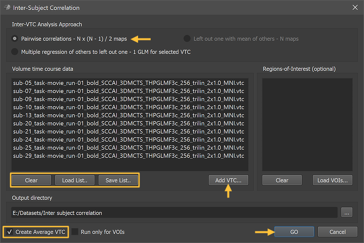
For whole-brain (voxelwise) analysis functional (VTC) files in a common (usually MNI or TAL) space need to be entered in the Volume time course data list box. This can be achieved by using the Add VTC button (see arrow above). Note that one can select in the appearing Open File dialog multiple VTC files in a folder. For later reuse the list of VTC files can be saved to disk usng the Save List button and later reloaded using the Load List button. The Clear button can be used to remove all entries from the list. In the example above, 10 VTC files (1 per included subject) have been added. It is important that the VTC files have the same number of volumes (time points) and that they are preprocessed in the same way.

ISC-Results1

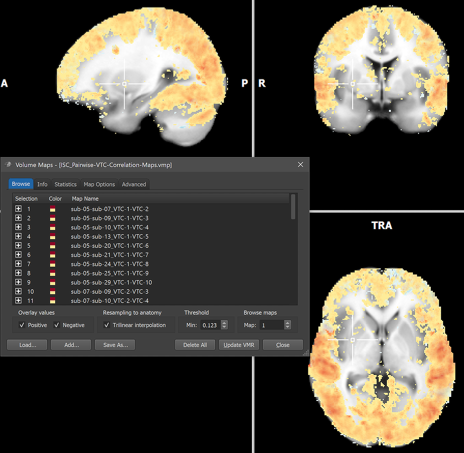
The ISC analysis can be started by clicking the GO button. The program will then calculated all (here pairwise) correlations at each voxel and stores the results as a series of maps to disk (e.g. 'ISC_Pairwise-VTC-Correlation-Maps.vmp'). In the pairwise approach N * (N-1) / 2 = 45 sub-maps will be generated in the example case (N = 10). The names of the individual maps in the appearing Volume Maps dialog (see screenshot above) indicate the respective pairing by the subject IDs (e.g. 'sub-05-sub-09' as well as by the index (row) of the respective files in the original VTC list (e.g. 'VTC-1-VTC-3'). To provide a first visual overview of the results, all individual correlation maps are selected (overlaid) as default. As usual, any individual map can be selected or any subset depending on the Map selection mode specified in the Advanced tab of the dialog.

Note. Calculating correct second-level statistical results for ISC analyses is, unvortunately, non-trivial and appropriate tools are currently implemented and planned to be available in a subsequent release. One of the main issues is that subjects are not contributing independent since each subject typically contributes to the first-level correlation estimation of every other subject. In the pairwise ISC approach, the resulting correlation coefficients are not statistically independent samples and, thus, violate the assumptions of parametric tests such as the t-test. Comparisons between groups using the traditional second-level approach below will produce largely correct results, especially for the leave-one-out ISC variant, since ISC-specific issues (such as non-independent samples) affect the data of the two groups in a similar way.

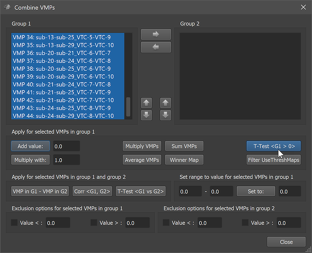
With these caveats in mind, a first impression of group results can be obtained using the Combine VMPs dialog (see below) that can be invoked using the Combine Maps button in the Advanced tab of the Volume Maps dialog. An average map can be calculated using the Average VMPs button that will average all maps selected in the first group; note that correlation values will be Fisher z-transformed and the resulting r value will be obtained by the inverse Fisher z-transform of the average z value. If all included functional files are from the same condition (e.g. all subjects watched the same movie), one can use the T-Test G1 > 0 button to calculate a t statistic at each voxel testing the null hypothesis that the correlation values of all (selected) maps are 0.0. In case that two conditions (e.g. two movies or two tasks) are used, the respective files can be statistically compared using the T-Test G1 vs G2 button after distributing them in the Group 1 and Group 2 list. Before processing the values, the

ISC-Results-Stat1

The figure below shows the resulting statistical t map that has been selected in the Maps list ([comparision group mean > 0] in the screenshot below). Note that the minimum threshold might be set to a very low value for a t statistic because the other (correlation) maps use values below 1. In the screenshot below, a minimum t value of 3.0 (and a maximum threshold of 10.0) has been selected.

ISC-Results-Stat2

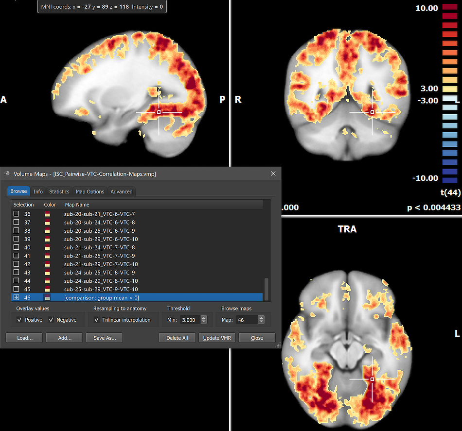
While both positive and negative values are selected in the Overlay values field (see screenshot above), only positive values are visible in the map (at the chosen threshold); this is expected for ISC analyses since the brains of the subjects are driven by the same stimulus sequence over time. As stated above, the results can, at present, only be used as a first indication of the results, proper statistical assessment will require more sophisticated testing procedures.

In case that the Create average VTC option had been selected in the Inter-Subject Correlation dialog, the respective output file will be stored in the specified output folder. Since noise and idiosyncratic effects are cancelled out in the average file (to an extent depending on the number of subjects), inspecting voxel or ROI time course fluctuations after linking this file to a VMR is very instructive since (large) fluctuations reveal common effects of the stimulus sequence across brains.